
Computer Vision: Eurosat Images Classification (Satellite Sentinel-2)
This project was developed using ".ipynb" files that were written in Portuguese, therefore, its repository contains the files in this same language.
To access the project repository, with all it's files in Portuguese, click HERE
The ".ipynb" used to develop the project is called "visao_computacional_projeto_final.ipynb". You can also click onto the Google Colaboratoy Link for project visualization
This page will present, in English, the project's goal, the process used to develop it and the results.
Project Goal
- The project has the goal to develop a Machine Learning Model that aims to classify RGB satellite images.
- The data was collected through Kaggle and it has 27.000 satellite images, Eurosat Dataset, with a GSD of 10m. The images were collected from the Sentinel-2 Satellite.
- Data Description:
- Image dimension: 64x64 pixels in RGB channels
- 10 class folders related to land use and coverage
- 19.000 training images and 8.000 validation/test images
Project Development
- The technical development of this project was divided into three phases:
- Data Load (images and metadata)
- Pre-processing data
- Model modeling
Data Load
- After loading the data, was noticed that the 27.000 were divided into 10 classes:
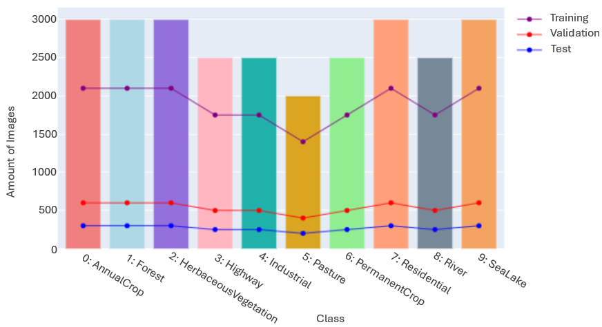
- Pasture (2.000 images)
- Residential (3.000 images)
- Industrial (2.500 images)
- SeaLake (3.000 images)
- HerbaceousVegetation (3.000 images)
- PermanentCrop (2.500 images)
- Highway (2.500 images)
- River (2.500 images)
- Forest (3.000 images)
- AnnualCrop (3.000 images)
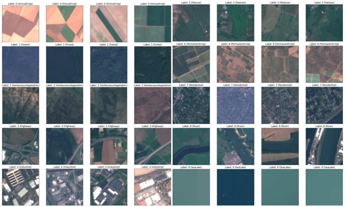
- The next image shows a mosaic with 4 images for each class
Pre-processing data
- The data Pre Processing was divided into phases:
- Separating images in three groups: training, validation and test
- Images visualization and problems they may present into the classification process
- Pytorch DataSet creation
- Pytorch DataLoad creation
- Calculation of pixel's Mean and Standard Deviation in each image group
- Initialize the Dataloader with the mean and standard deviation that were obtained
- Dataload images observation
Modeling
- Regarding the project's modeling, it can be fragmented into four phases:
- CNN Model creation (CNN was the one chosen to do the image classification)
- Definition of hyperparameters and relevant metrics
- Definition of the process necessary to train the model
- Model Training
Results
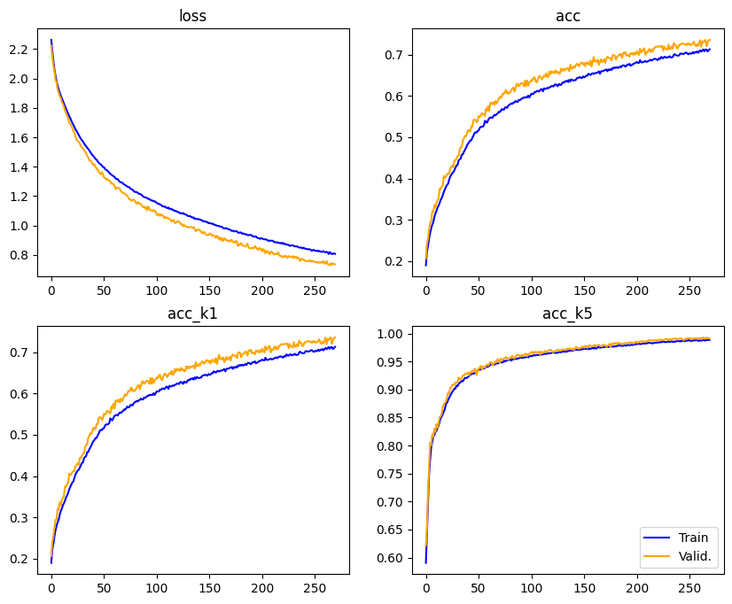
Accuracy and Loss Graph during training and validation
- With those graphs, it is possible to observe that the accuracy values have a tendency to grow without presenting overfitting.
- We observe the values to top-1 and top-5 accuracy.
- TOP-1 Considers the accuracy to the element that presents bigger prediction value
- TOP-5 Considers the accuracy to the top 5 elements that presents bigger prediction value
- A difference regarding TOP-1 and TOP-5 is that, during the firsts Epochs the top-5 has a significant accuracy peak, reaching satisfactory values. If this was the main form of analysis, it would not be necessary so many epochs to achieve a good result.
Accuracy, Recall and Precision in top-1 and top-5
- As observed in the last topic, it is possible to conclude that in most of the cases, the real class within the 5 that presents bigger probability of being it.
- If only considered the TOP-1 accuracy the project presented good results (not as good as the top-5).
- TOP-1: the model classified correctly 1959 images out of 2700 in the test phase.
- TOP-5: the model classified correctly 2676 images out of 2700 in the test phase.
| Metrics | TOP-1 | TOP-5 |
|---|---|---|
| Total Accuracy | 0.73 | 0.99 |
| Total Precision | 0.69 | 0.99 |
| Total Recall | 0.69 | 0.99 |
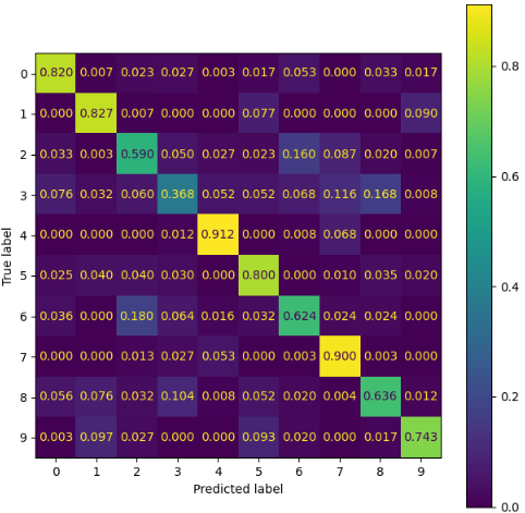
Confusion Matrix to results Analysis
- The confusion matrix was developed for the TOP-1 accuracy case.
- Therefore, the cases in place are the ones where the image in result had the bigger probability to occur, regarding the real TARGET value.
- The confusion matrix presents True Label X Predicted Label
- It is possible to analyse the predicted class distribution in comparison with its true label
- The class that presented higher prediction difficulty was 3, being mostly confused as the classes 7 and 8.
- The second class that presented higher prediction difficulty was 2, being mostly confused as class 6, which was also confused with class 2.
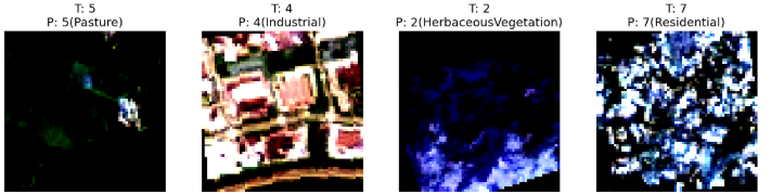
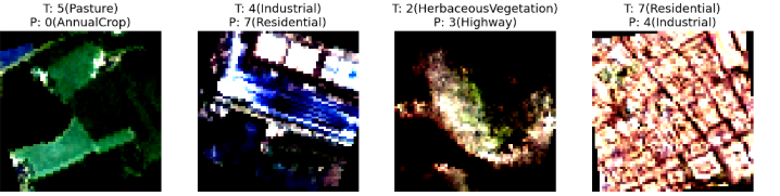
Correct and Incorrect Predicted Images Visualization
- The images that were predicted incorrectly didn't have a good image delimitation or presented a characteristic that would be similar to other classes, making the model confused.
- In the images, P indicates the predicted label, while T the true label
- Images Classified Correctly:
- Images Classified Incorrectly:
Conclusion
- The project presented good accuracy values, over 70%
- For this project, the different amount of images per class did not affect the final result. The class with the least amount of images, 5 (2000 images), presented better results regarding the confusion matrix
- Although, if there were more images, the model could have developed better in the classes where it did not present good results
- In the beginning of the project, it was observed that there would probably occur a confusion between the classes "3" and "8" (Highway and River), because, visually, they have similar characteristics. This idea was confirmed after the results were obtained.
- In general, the model obtained satisfactory results in classifying images. However, if the goal is to focus in specific cases, such as the class 3, for example, maybe it is better to try another model architecture that will satisfy this class in a better way.
- Finally, if the idea is to use the model to a more general classification, analysing top-5, it has a great applicability with the accuracy close to 100%.