
Plotly & Pandas: Movie Data Visual Analysis
This project was developed using ".ipynb" files that were written in Portuguese, therefore, its repository contains the files in this same language.
To access the project repository, with all it's files in Portuguese, click HERE
The ".ipynb" used to develop the project is called "plotly_pandas_movies_visual_analysis.ipynb". You can also click onto the Google Colaboratoy Link for project visualization
This page will present, in English, the project's goal, the process used to develop it and the results.
Project Goal
- The project has the goal to apply a descriptive analysis of a "Movie Lens Data"
- The data was collected through "Group Lens" and its "movielens" "ml-100k/" files.
- The files used during the project were: u.data; u.item and u.user
- This Project was developed during the Post-graduation in Deep Learning course and as Question and Answer format. Therefore, the project was organized in order to answer the questions that were made, using the PLOTLY and PANDAS python libraries.
- Finally, this project main goal was to develop knowledge in PANDAS and PLOTLY libraries
Project Development
- The technical development of this project was divided into data load, followed by it's 2 phases (2 main questions):
- Presentation in visual format (using Plotly) of Minessota's data files
- DataFrame manipulation using Pandas
Data Load
- For the project, the only data necessary were the three mentioned before in the "Project Goal" section
- The data contains user rating related to a specific type of movie within the three .csv files. The analysis made are related to the specification of each file and integration between them.
- In each description, there is an example of the data
- Data Description:
- u.data: contains the relation between user, movie and the rate given, such as: user_id; movie_id; rating; timestamp
user_id movie_id rating timestamp 22 377 1 878887116 186 302 3 891717742 - u.item: contains movie information, such as: movie_id; movie_title; release_date; video_release_date; IMDb_URL; movie's genre
movie_id movie_title release_date video_release_date IMDb_URL unknown Action ... Thriller War Western 1 Toy Story (1995) 01-Jan-1995 NaN http://us.imdb.com/M/title-exact?Toy%20Story%2... 0 0 ... 0 0 0 2 GoldenEye (1995) 01-Jan-1995 NaN http://us.imdb.com/M/title-exact?GoldenEye%20(... 0 1 ... 1 0 0 - u.user: contains the user information, such as: user_id; age; gender; occupation; zip_code
user_id age gender occupation zip_code 1 24 M technician 85711 2 53 F other 94043
- u.data: contains the relation between user, movie and the rate given, such as: user_id; movie_id; rating; timestamp
- To better analyse the data, in further steps, the different .csv files will be joined by the user or movie ID
Presentation in visual format (using Plotly) of Minessota's data files
Visual representation of every categorical information
- Each one of the three separated data (users, data and item) has different categorical items, therefore, it analysis was made separating one another
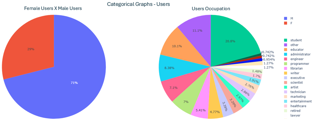
- u.user (Users):
- The two categorical data found were: gender and occupation
- The image below shows the visual information regarding those items
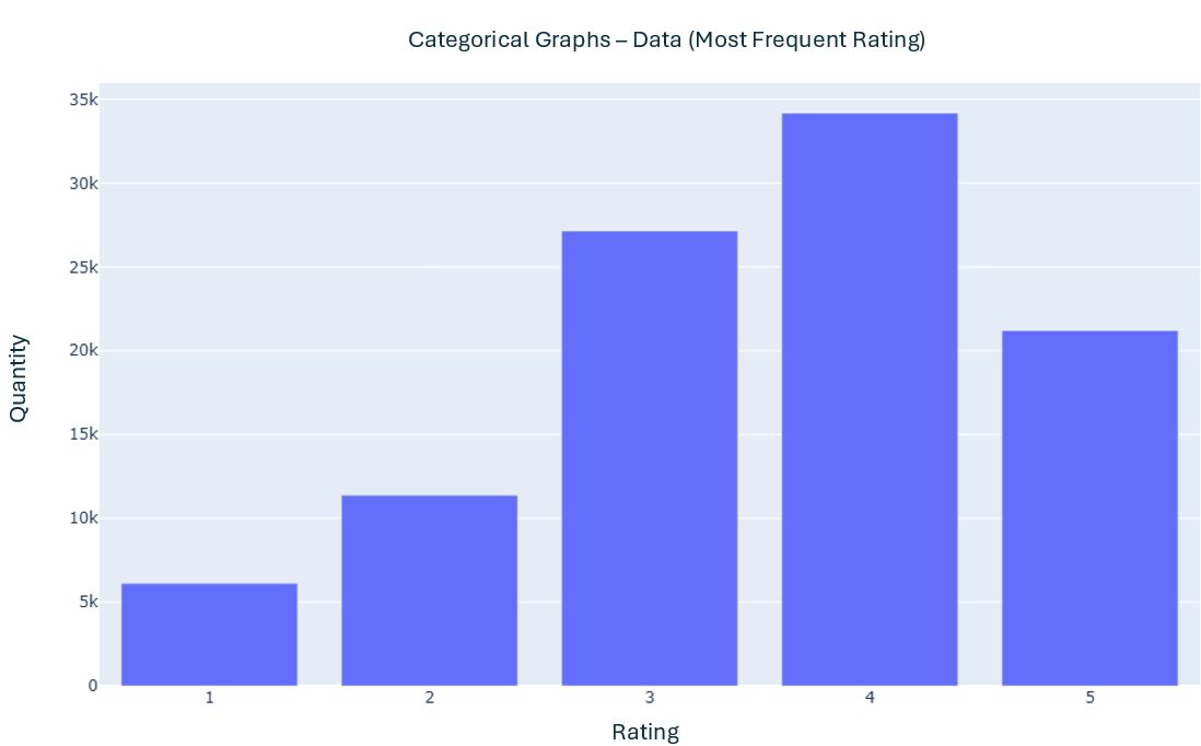
- u.data (Rating per user):
- The only categorical data found important to present a graph at this moment was: rating
- The users and movies ids are also categorical data. It would be possible to either group them by movie or by users. This would allow an observation such as: Chose a single user and see the movies they ranked. This analysis was not done in the moment.
- The image below shows the visual information regarding the rating
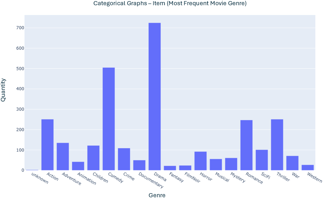
- u.item (Movies Information):
- For this data, the categorical data identified worth demonstration was movie gender
- A single movie can contain one or more genders
- The image below shows the visual information regarding the gender
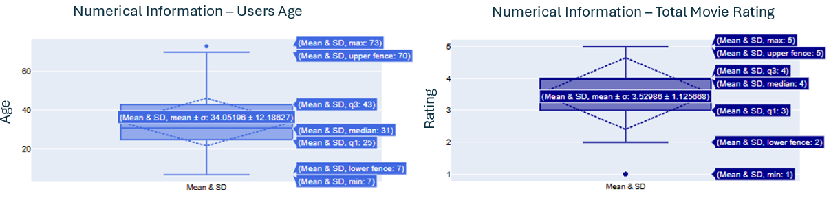
Value Information regarding numerical data
- In this phase, it was obtained the numerical value for each numerical data.
- Those values were: maximum, minimum, mean, median, and STD
- The image below shows the visual information regarding those values for: age (user information); rating (data information)
Creation of time graphs related to the data
- In this phase, two graphs were created with the goal to analyse data through time
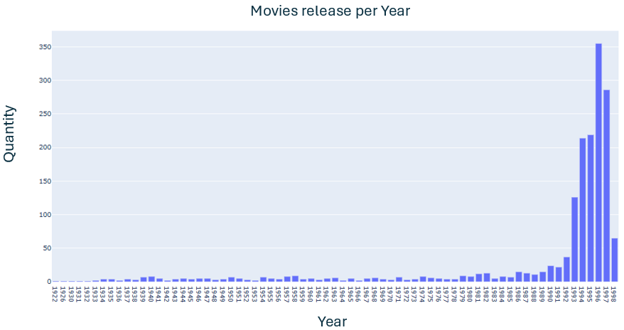
- The first graph represents the release of movies, starting in 1922 and ending in 1998
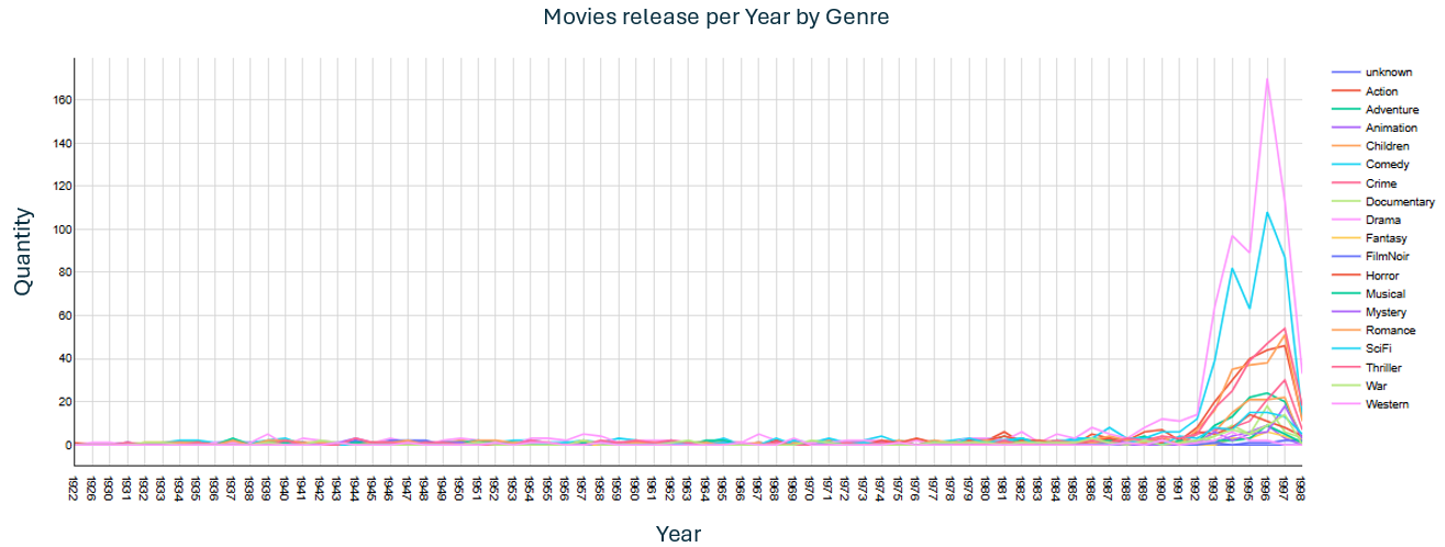
- The second graph represents the release of movies by genre, starting in 1922 and ending in 1998
- From the second graph it is possible to visualize a huge increase in the Drama section followed by Comedy, compared to the others, especially after 1992
Rating Analysis (by user gender and movie genre)
- In this phase, two more graphs were created in order to better understand the data
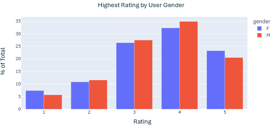
- The first graph analyzed the rating by different user's gender
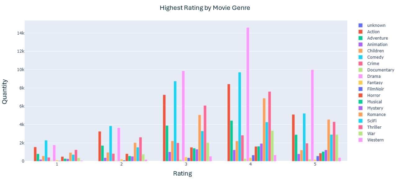
- The second graph analyzed the rating by different movie's genre
- The goal was to analyse if the rating was influenced by gender or movie genre
- In conclusion, the average rating given by male and female was very similar with women giving more 1 and 5 scores, and man the main responsible for the other ones.
- Regarding movie genre, the rating follows a pattern related to the total amount of each genre that exists. Even so, some aspects are interesting: There are more Drama then Comedy movies, but there are more Comedy movies with 1 and 2 scores, comparing to Drama.
DataFrame manipulation using Pandas
- This final phase focused on manipulate the DataFrames by working with pandas elements
- The first manipulation made was the generation of a new DataFrame with only "Male" and "Student" users that are over 20
- A function was applied into the USER dataset:
student_users = users[(users.age > 20)&(users.occupation == "student")&(users.gender == "M")] - The table below presents a fraction of the new DataFrame that was generated
user_id age gender occupation zip_code 9 29 M student 01002 33 23 M student 27510 73 24 M student 41850
- A function was applied into the USER dataset:
- The second manipulation made was to discover the amount of female programmers
- A function was applied into the USER dataset:
programmer_F_users = users[(users.occupation == "programmer")&(users.gender == "F")] - It was found a total of 6 users that fit the criteria
- A function was applied into the USER dataset:
- The last manipulation made was to discover the amount of rating over 3
- A function was applied into the DATA dataset:
over3_data = data[data.rating > 3] - Results per rating (4 and 5): Rating 4 with 34.174 units; Rating 5 with 21.201 units
- It was found a total of 55.375 ratings over 3
- A function was applied into the DATA dataset: